1. Introduction
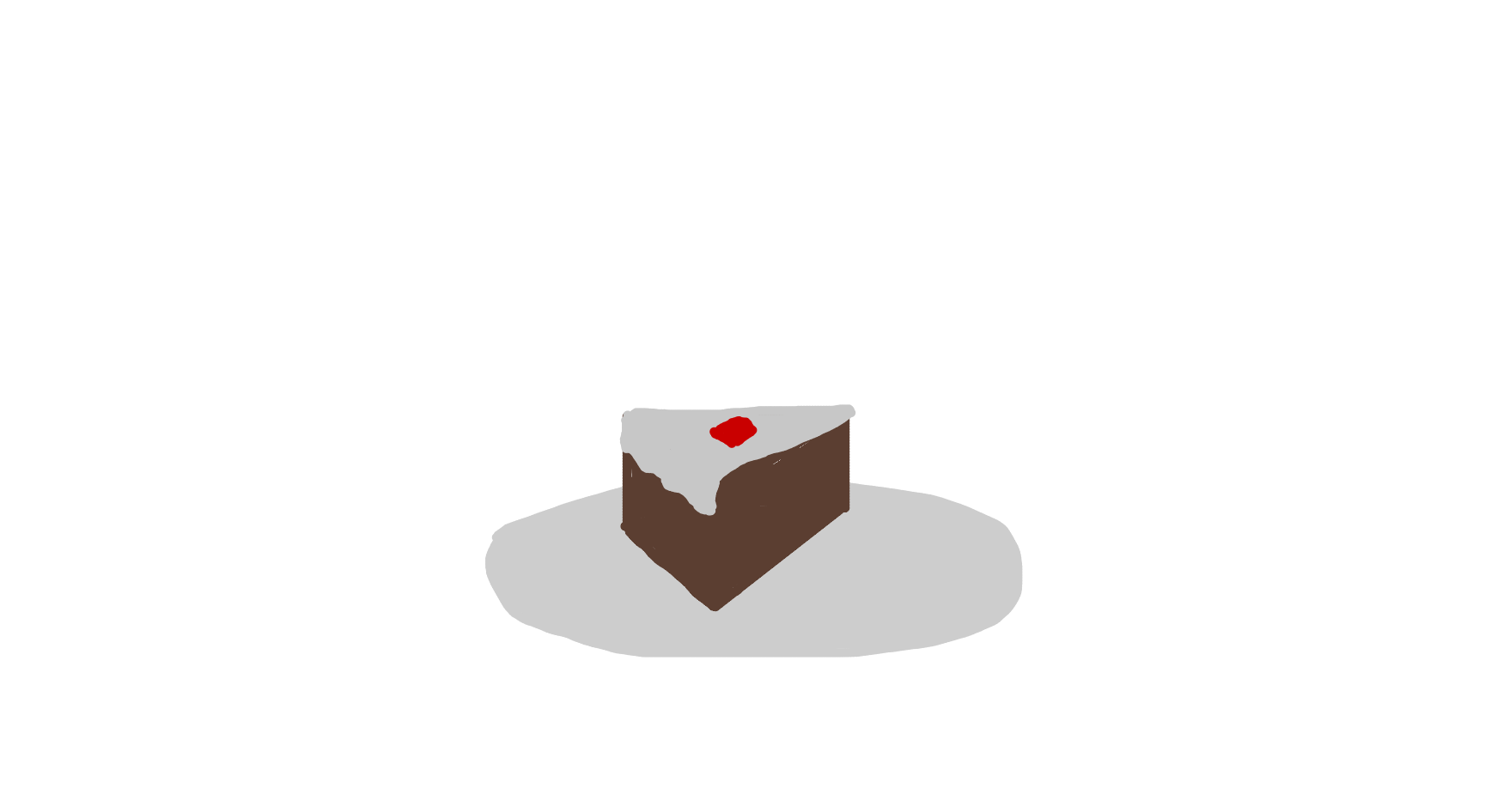
Let’s set the scene. I (16M) am a huge fan of Minecraft. As such, since my birthday is coming up, I obviously want to get a Minecraft themed birthday party - this will include a pig pinata, Minecraft themed utensils, and obviously, a Minecraft cake.
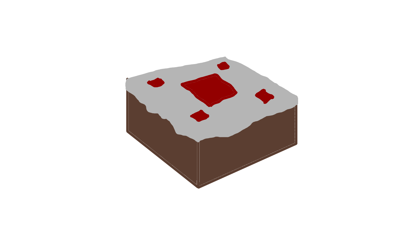
A wonderful Minecraft cake.
When it comes time to cut the cake, I’ve only got a couple of - relatively self explanatory - rules. Obviously, I want every cut of the cake to be a triangle (for the sake of tradition), and I want every single cut to have an equal area, to avoid situations like this.
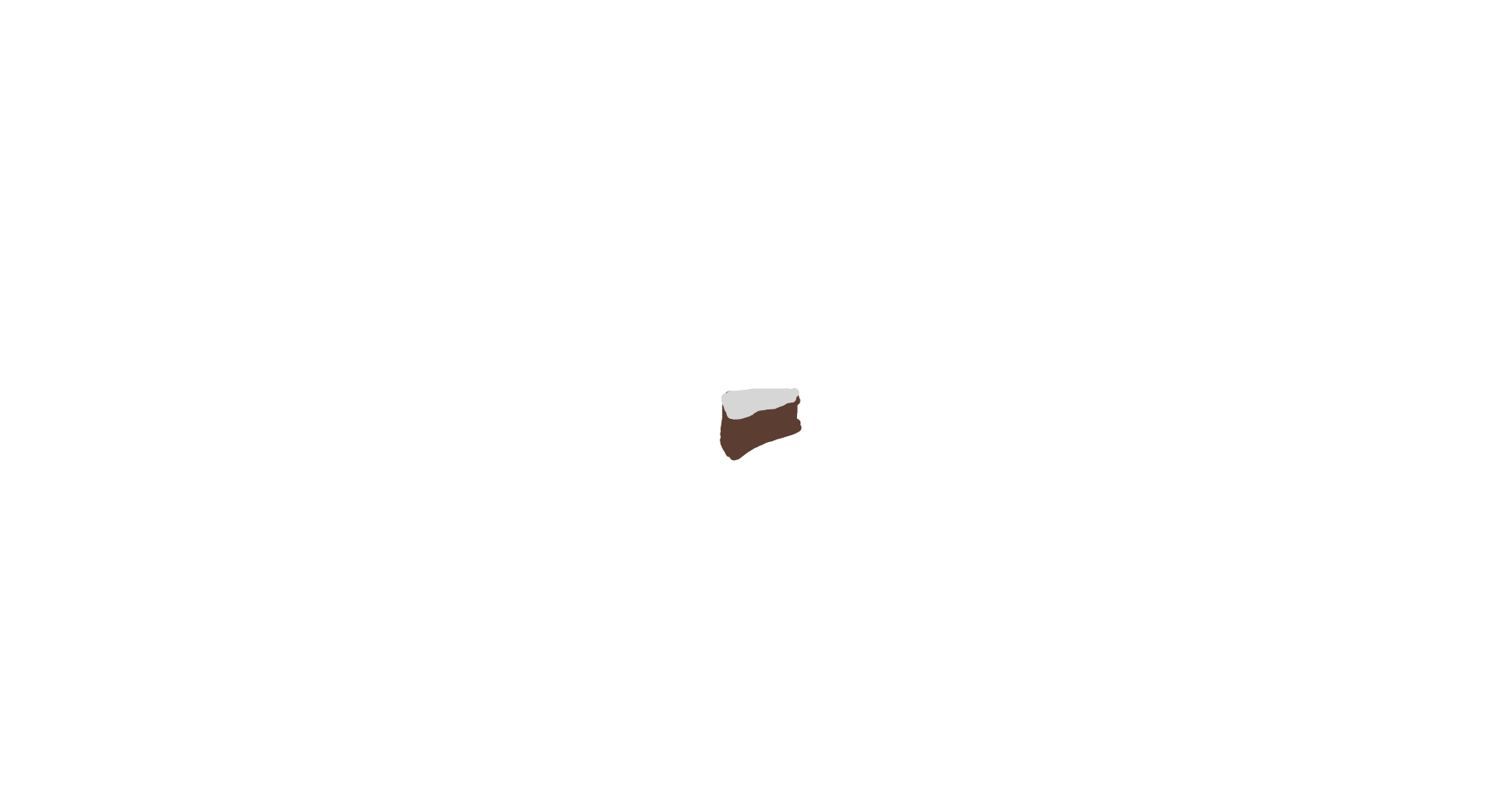
He got slightly less cake.
I invited six people other than me to my birthday party. How should I cut the cake?
At a first glance, it seems like there has to be a solution. I mean, there’s an infinite variety of ways to cut a cake into \(7\) triangles - surely one of them is such that all the triangles have equal area, right?
In fact, I encourage you to give this problem a shot! Try to split a square into \(7\) equal pieces, and come back when you’re done (or you give up).
…
If you’re back, I’m pretty sure you’ve given up - because it’s actually impossible! You might not have expected it, but there’s no possible way to split up a square into \(7\) triangles of equal area.
In fact, more generally, there’s no possible way to split up a square into an odd number of triangles with equal area. The first time I saw this result - known as Monsky’s Theorem - I was mindblown. Out of all the odd numbers, there’s not a single one that this property holds for? It sounds absurd!
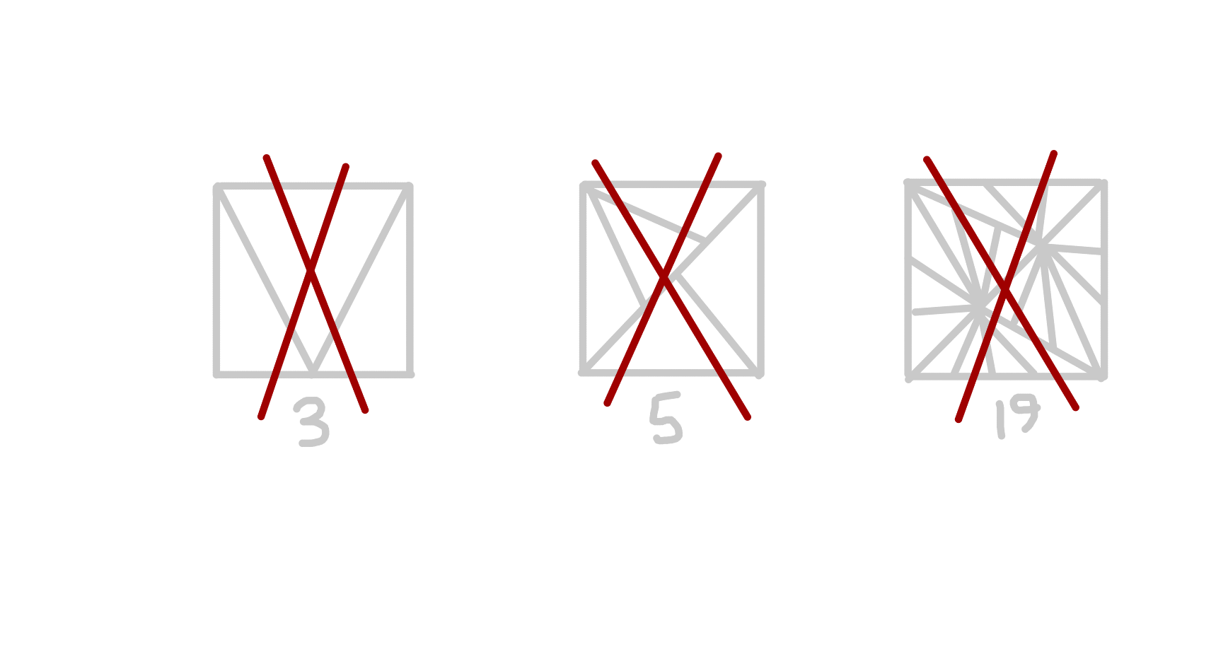
It just doesn't work.
And yet, the proof of this theorem connects areas of mathematics in ways I never thought possible. This simple geometry problem draws from the far-reaching fields of algebraic number theory and graph theory to create an incredibly beautiful solution. So, join me, as we attempt to uncover the secrets behind Monsky’s theorem.
This post is heavily inspired by this presentation from SUMO - if you would like to see a compressed version of the process we follow below, you can visit their lecture notes.
2. Exploration
You might’ve noticed that the statement only talks about an odd number of triangles. What about an even number of triangles?
Well, let’s start with the smallest even number - \(2\). Splitting a rectangle into \(2\) triangles of equal area is easy, since all you have to do is cut it along the diagonal.
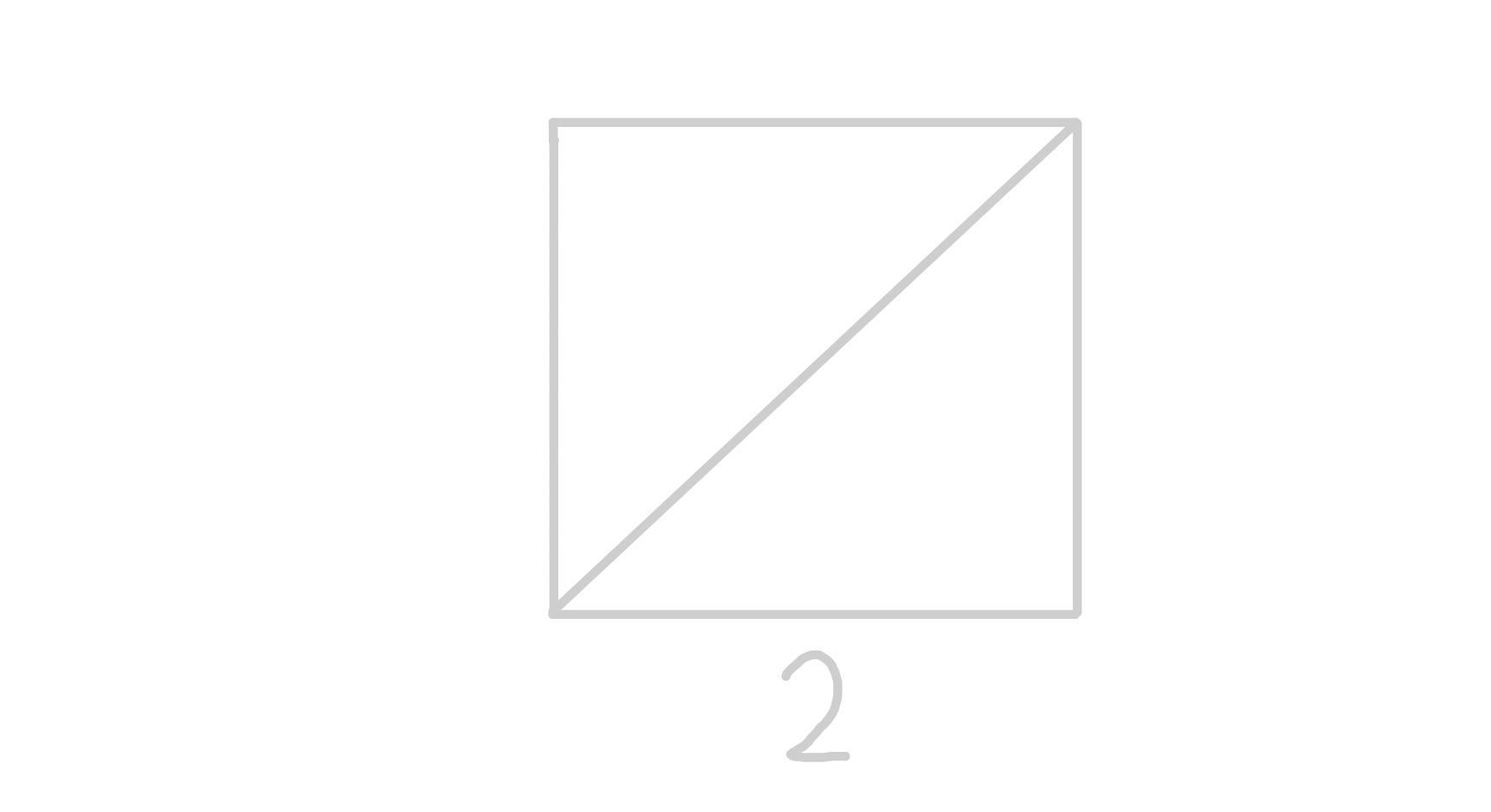
2 triangles is easy.
This basic observation actually gives us a way to cut a square into any even number of triangles. See, it’s relatively easy to find a way to split up a single triangle into \(n\) equal area triangles for any \(n\) - just split up the base up into \(n\) equal parts.
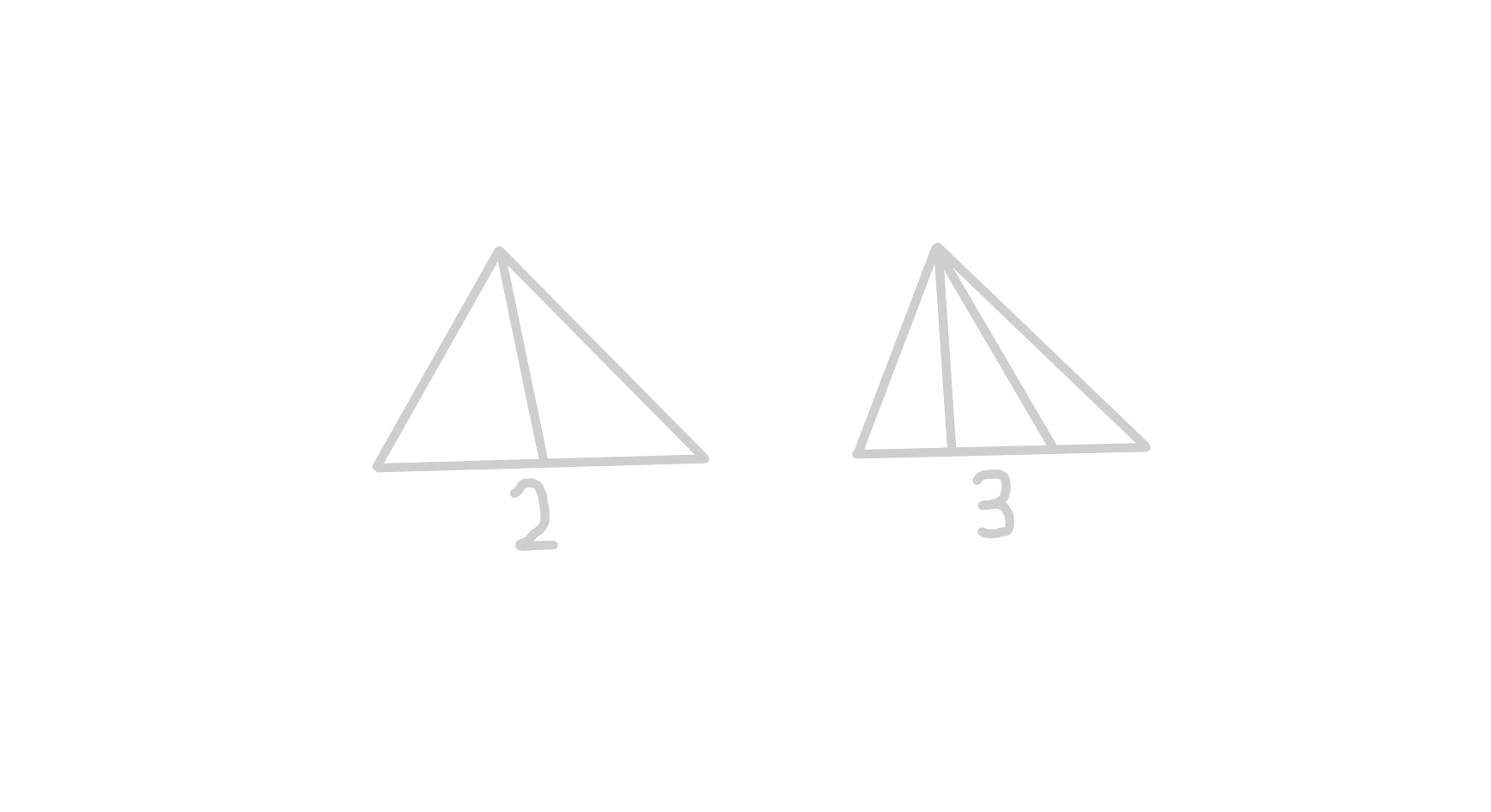
Splitting up triangles is easy.
So, since we already have \(2\) triangles, we can just split them each up into \(n\) individual parts to get \(2n\) total equal area triangles for our square. For example, here’s how you would find \(8\) equal area triangles in the square.
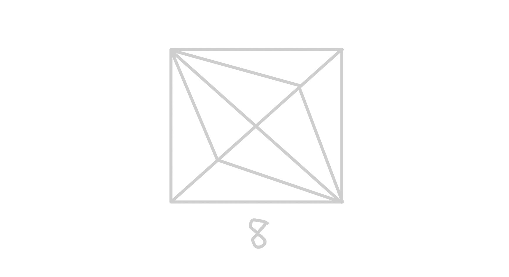
8 triangles is easy.
Now that that’s done with - and you hopefully are a little more familiar with triangulations - let’s get into the main problem at hand.
What do we know about triangulations? Well, we know that we have \(n\) triangles in the triangulation (for some odd number \(n\)), and we can assume that we’re trying to split up a unit square, because scaling doesn’t matter. These two pieces of information combined tell us that the area of each triangle is \(\frac{1}{n}\).
Since that’s really all we have to go off right now, we can do a short review of some of the most common ways to find the area of a triangle. There’s:
- The traditional area formula - a triangle with base length \(b\) and height \(h\) has area \(\frac{1}{2}bh\).
- The \(\text{sin}\) area formula - a triangle with angle \(\theta\) in between sides of length \(a\) and \(b\) has area \(\frac{1}{2} ab \sin(\theta)\).
- Heron’s formula - a triangle with sides \(a, b, c\) has area \(\sqrt{s(s-a)(s-b)(s-c)}\), where \(s\) is the semiperimiter \(s = \frac{a + b + c}{2}\).
- The Shoelace formula - a triangle with vertex coordinates \((x_1, y_1), (x_2, y_2), (x_3, y_3)\) has area \(\frac{\|x_1y_2 + x_2y_3 + x_3y_1 - x_2y_1 - x_3y_2 - x_1y_3\|}{2}\).
Of course, there are other ones (\(\frac{abc}{4R}\), anyone?) but these are the primary 4.
Which of these is the best to use given the situation at hand? Well, we want to pick the formula that allows for the least amount of information from the triangulation as possible, since the more information we take from the triangulation, the more variables we have to deal with.
Knowing this, the traditional area formula is probably a bad idea, because we would have to keep track of both bases and heights. Similarly, the angle formula is a bad idea, because we have to keep track of both angles and lengths.
Heron’s formula doesn’t seem like a bad choice, because we only have to keep track of one value: the lengths. Similarly, the Shoelace theorem also only requires one value: the coordinates of the vertices.
Choosing between the two all comes down to one thing - specificity. Knowing the lengths of the sides of all triangles in a triangulation doesn’t tell us much about the triangulation itself. On the other hand, knowing what coordinates the vertices are on tells us a whole lot about the triangulation - in fact, it allows us to reconstruct it completely!
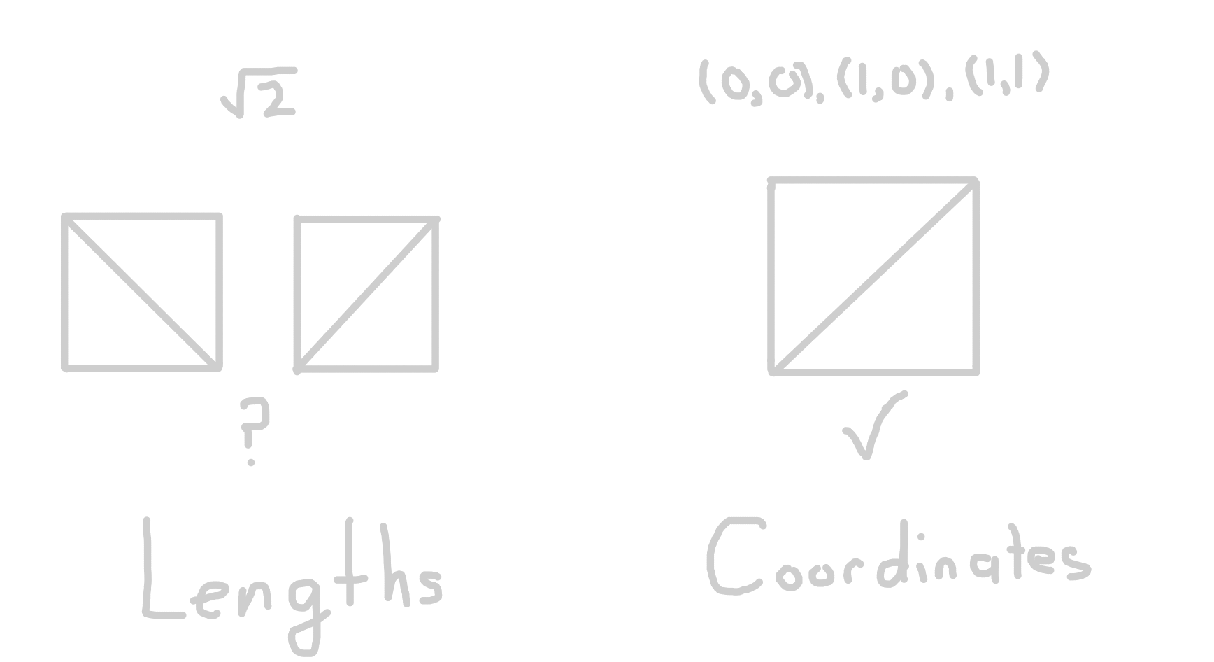
Shoelace is much more specific than Heron's.
So, now we know that for any triangle in the triangulation with vertices \((x_1, y_1), (x_2, y_2), (x_3, y_3)\), we have the relation
\[\frac{\|x_1y_2 + x_2y_3 + x_3y_1 - x_2y_1 - x_3y_2 - x_1y_3\|}{2} = \frac{1}{n}\]
In fact, we can simplify this greatly for a very specific triangle in the triangulation. Note that \((0, 0)\) is one of the vertices of the unit square - as such, it must be one of the vertices for at least one of the triangles in the triangulation.
Therefore, for the triangle with vertices \((0, 0), (a, b),\) and \((c, d)\), we can rewrite the Shoelace theorem’s statement as
\[\frac{\|ad - bc\|}{2} = \frac{1}{n} \implies \|ad - bc\| = \frac{2}{n}\]
[To those of you that know linear algebra, this expression should look very familiar. See if you can figure out why by drawing the triangle out and recalling the geometric definition of the determinant!]
Now, we get our first inkling of why the triangulation might work for even \(n\), but not for odd \(n\). It seems like for even \(n\), that factor of \(2\) at the top will cancel, but for odd \(n\), it won’t. Maybe some sort of divisibility idea would work?
But \(a, b, c,\) and \(d\) are between \(0\) and \(1\), and you can’t work with divisibility over the rational numbers. Right?
3. The 2-adic norm
For the sake of this problem, we won’t need to discuss the full extent of the \(p\)-adic numbers - instead, we’ll focus on a very specific part of them, namely the \(2\)-adic norm (a special case of the \(p\)-adic norm). If you’re interested in learning more after reading this blog post, there are plenty of good resources online where you can learn a lot about the \(p\)-adic numbers in general.
The \(2\)-adic norm is defined over the rational numbers (all fractions, essentially), as follows:
For every rational number \(a\), there exists an integer \(n\) such that \(a = 2^n \cdot \frac{p}{q}\) where both \(p\) and \(q\) are odd. The \(2\)-adic norm of a (written as \(\|a\|_2\)) is equal to \(2^{-n}\).
For example, \(\|\frac{1}{2}\|_2 = 2\), because \(\frac{1}{2} = 2^{-1} \cdot \frac{1}{1}\). \(\|\frac{2}{3}\|_2 = \frac{1}{2}\), since \(\frac{2}{3} = 2 \cdot \frac{1}{3}\).
There’s a couple important properties of the \(2\)-adic norm. They are as follows:
- The \(2\)-adic norm is nonnegative - so \(\|a\|_2 \geq 0\) for all real \(a\). This is obvious, since \(2^{-n} \geq 0\) for all \(n\).
- The \(2\)-adic norm is definite - namely, \(\|a\|_2 = 0\) implies \(a = 0\). In fact, \(\|0\|_2\) is defined as \(0\) in order to make this valuation consistent with the properties shown below, which are pretty important.
- The \(2\)-adic norm is multiplicative - namely, \(\|ab\|_2 = \|a\|_2 \cdot \|b\|_2\). This is also clear from the definition.
- The 2-adic norm satisfies the ultrametric inequality, so \(\|a + b\|_2 \leq \text{max}(\|a\|_2, \|b\|_2)\). This can be proven relatively easily - give it a shot if you want to get used to the \(2\)-adic norm!
These properties combined make the \(2\)-adic numbers (the real numbers with the distance being the \(2\)-adic distance instead of the normal one) into a space known as an ultrametric space.
A visualization of the 2-adic numbers (from Wikipedia).
The astute among you might have noticed a slight issue with our use of the \(2\)-adic metric, and that’s the fact that we’re assuming that \(a, b, c,\) and \(d\) are rational numbers. This isn’t necessarily a valid assumption, though - in fact, \(a\) could very well be something like \(\frac{\sqrt{2}}{2}\). So how are we supposed to use the \(2\)-adic norm now?
Well, luckily for us, there’s a theorem that solves all of our problems. Essentially, the theorem states that there’s a unique norm over the real numbers that matches our desired \(2\)-adic norm for every rational number. You can think of this as a sort of “extension” of the \(2\)-adic norm from the rationals to the reals. The details of the proof are pretty complicated (way more than could fit into a single blog post) - if you’re up for the challenge, there’s a proof in Lang’s algebra.
So, how does this help us? Well, remember that we want to show that \(\|ad - bc\|\) is not equal to \(\frac{2}{n}\) for any odd \(n\). Therefore, if we take the \(2\)-adic norm of both sides and show that those are not equal, we’re done!
The \(2\)-adic norm of the right side is \(\|\frac{2}{n}\|_2 = \frac{1}{2}\). Therefore, we just have to show that \(\|ad - bc\|_2\) is not equal to \(\frac{1}{2}\). It would make a lot of sense that the \(2\)-adic norm would be on one side of that value - either greater than or less than it. Let’s assume for now that it needs to be greater than \(\frac{1}{2}\) (because that allows for a greater variety of values) - this essentially means that we must have \(\|ad - bc\|_2 \geq 1\).
What requirements should we have for \(a, b, c,\) and \(d\) for this inequality to hold true? Well, since we see subtraction, we might be reminded of the ultrametric inequality - that \(\|ad - bc\|_2 \leq \text{max}(\|ad\|_2, \|bc\|_2)\) (remember that negatives don’t matter for \(2\)-adic norms!).
This inequality is facing the wrong way, though. We want to show that \(\|ad-bc\|_2\) is greater than something, not less than it! So, we can instead utilize a different form of the equality - namely, we can write it as \(bc + (ad - bc) = ad\). Applying the ultrametric inequality to this gives us \(\|ad\|_2 \leq \text{max}(\|ad - bc\|_2, \|bc\|_2)\).
To get this into the form we want, we would normally need to have \(\|bc\|_2 \leq \|ad - bc\|_2\) (so that there’s a \(\|ad - bc\|_2\) on the right side of the ultrametric inequality). However, there’s no easy way to confirm that this is true.
Instead, there’s actually a more elusive way to confirm that the \(\|ad - bc\|_2\) is the one on the right side, and it’s to instead require that \(\|bc\|_2 < \|ad\|_2\)! Why does this work? Well, assume for the sake of contradiction that \(\|bc\|_2\) is the term that ends up on the right side; then, we would have to have \(\|ad\|_2 \leq \|bc\|_2\), which contradicts our assumption! Therefore, the \(\|ad - bc\|_2\) term must be the one on the right side, as desired!
So, we now have our first requirement - that \(\|bc\|_2 < \|ad\|_2\). Since we have that \(\|ad - bc\|_2 > \|ad\|_2\), the only requirement left is to make sure that the right side is greater than \(1\) - alternatively, that \(\|a\|_2 \geq 1\) and \(\|d\|_2 \geq 1\) (by the multiplication property). [This is a looser requirement than the original, yes - however, it should suit our purposes.]
So, these are our two assumptions. \(\|a\|_2 \geq 1, \|d\|_2 \geq 1,\) and \(\|bc\|_2 < \|ad\|_2\). Let’s call points of the type \((a, b)\) blue points, and points of the type \((c, d)\) green points. Namely, blue points satisfy the requirement \(\|a\|_2 \geq \text{max}(1, \|b\|_2)\), and green points satisfy the requirement \(\|d\|_2 > \text{max}(1, \|c\|_2)\).
Let’s call every point that’s not blue or green a red point. This gives us \(3\) colors of points with which we can color the unit square. For a couple examples, the point \((0, 0)\) is pretty obviously a red point, since \(\|0\|_2 = 0\). \((1, 1)\) is a blue point (because of the greater than or equal to), \((0, 1)\) is a green point, and \((1, 0)\) is a blue point.
A (relatively accurate) coloring of the unit square is provided below.
A (low-res) coloring of the plane.
Now, you might be able to notice a pretty obvious problem. Our argument requires for there to be a triangle with one vertex as \((0, 0)\), and the other two vertices blue and green, respectively. However, it’s now becoming pretty clear that there doesn’t necessarily have to be a blue and green point in the triangulation - I’m sure you could find a triangulation that doesn’t satisfy those requirements.
So, does that mean this line of thought is dead? Do we have to go back to the drawing board?
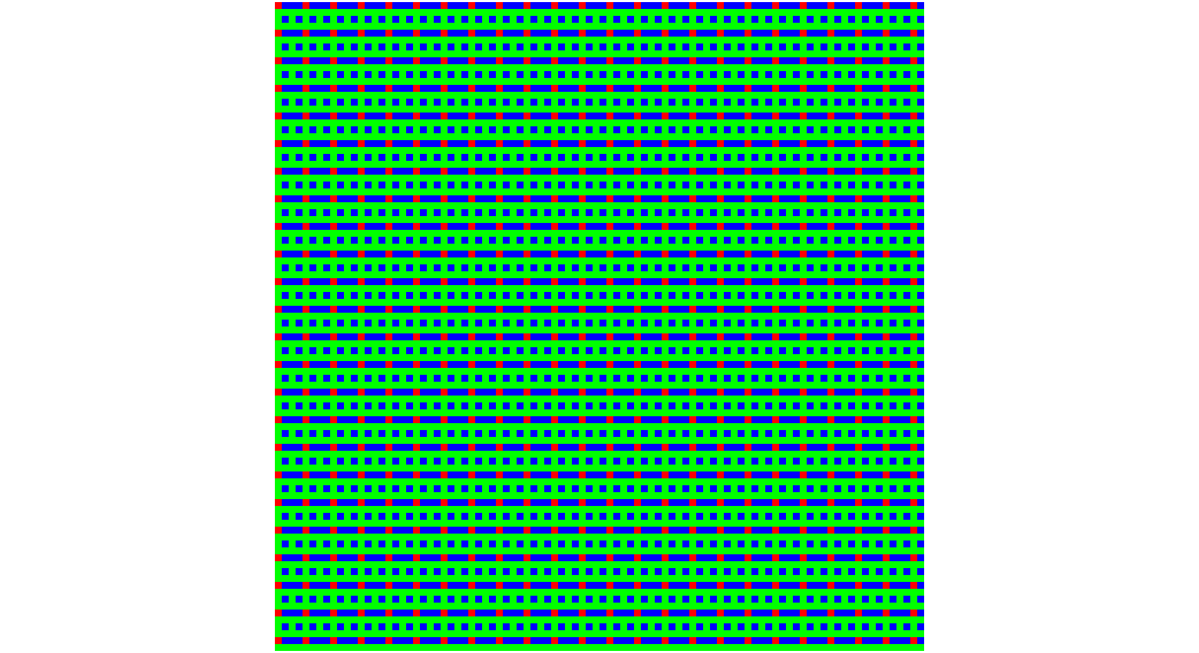
Well, let’s not be so hasty. We know that although the triangle corresponding to \((0, 0)\) doesn’t necessarily have a blue and green vertex, some of the other triangles might. If we could somehow shift those triangles back to \((0, 0)\), then we could still use our approach just fine.
What if we shifted triangles?
Additionally, unlike with a traditional distance metric, we’re using a \(p\)-adic norm here. \(p\)-adic norms lose a lot of information by choosing to focus only on the powers of a certain prime that correspond to the point at hand - this means that two completely different points could possibly have the same \(p\)-adic representation. This means that even after shifting, the \(p\)-adic norms of the points could stay the same - this would be our ideal scenario.
So, what should we consider shifting? Well, we know that \((0, 0)\) is a red point - if we want to preserve blue and green points, maybe we could shift the red point to another red point?
First, though, we should probably find a concrete description of the red points. If it’s not a blue point, then we either have \(\|a\|_2 < 1\) or \(\|a\|_2 < \|b\|_2\). And if it’s not a green point, then we must have \(\|b\|_2 \leq 1\) or \(\|b\|_2 \leq \|a\|_2\). Obviously, both of the latter constraints can’t be true, so one of the former ones has to be true. Let’s assume for now that \(\|a\|_2 < 1\) - then, no matter whether \(\|b\|_2 \leq 1\) or \(\|b\|_2 \leq \|a\|_2\) is true, we have \(\|b\|_2 \leq 1\). A similar argument holds if we choose \(\|b\|_2 \leq 1\) to be true - this means that the red points are exactly the set of points with \(\|a\|_2 < 1\) and \(\|b\|_2 \leq 1\)!
Let’s say that we want to shift a red point \((a, b)\) to \((0, 0)\). Then, every other point \((x, y)\) will be taken to the point \((x - a, y - b)\). In fact, this transformation will maintain the color of the point! [You might’ve been able to predict this by looking at how periodic the coloring of the plane is!]
For example, if \((x, y)\) was a red point, then \(\|x - a\|_2 \leq \text{max}(\|x\|_2, \|a\|_2) < 1\) (because both \((x, y)\) and \((a, b)\) are red points), and a similar argument holds for \(\|y - b\|_2\) - therefore, \((x - a, y - b)\) is also red. Similar arguments hold for the other two cases as well - see if you can figure them out!
So, if we can just find a triangle with all \(3\) colors on the vertices, we’re done! We just have to shift the red vertex to \(0\), and then we can use the Shoelace argument above to show that such a triangle must be impossible!
At a first glance, the claim that every single triangulation must have a tricolor triangle doesn’t seem much more believable than our first claim. However, I encourage you to try for a couple minutes to find a counterexample! Once again, you’ll find that you can’t.
As it turns out, this is the point at which we must make our second connection. In fact, if you’re a fan of graph theory, you probably already know where we’re going with this!
4. Sperner’s Lemma
First, I’ll give a brief overview of graph theory, and then we’ll see how to apply it to the problem at hand. If you already know the basics of graph theory, feel free to skip this section.
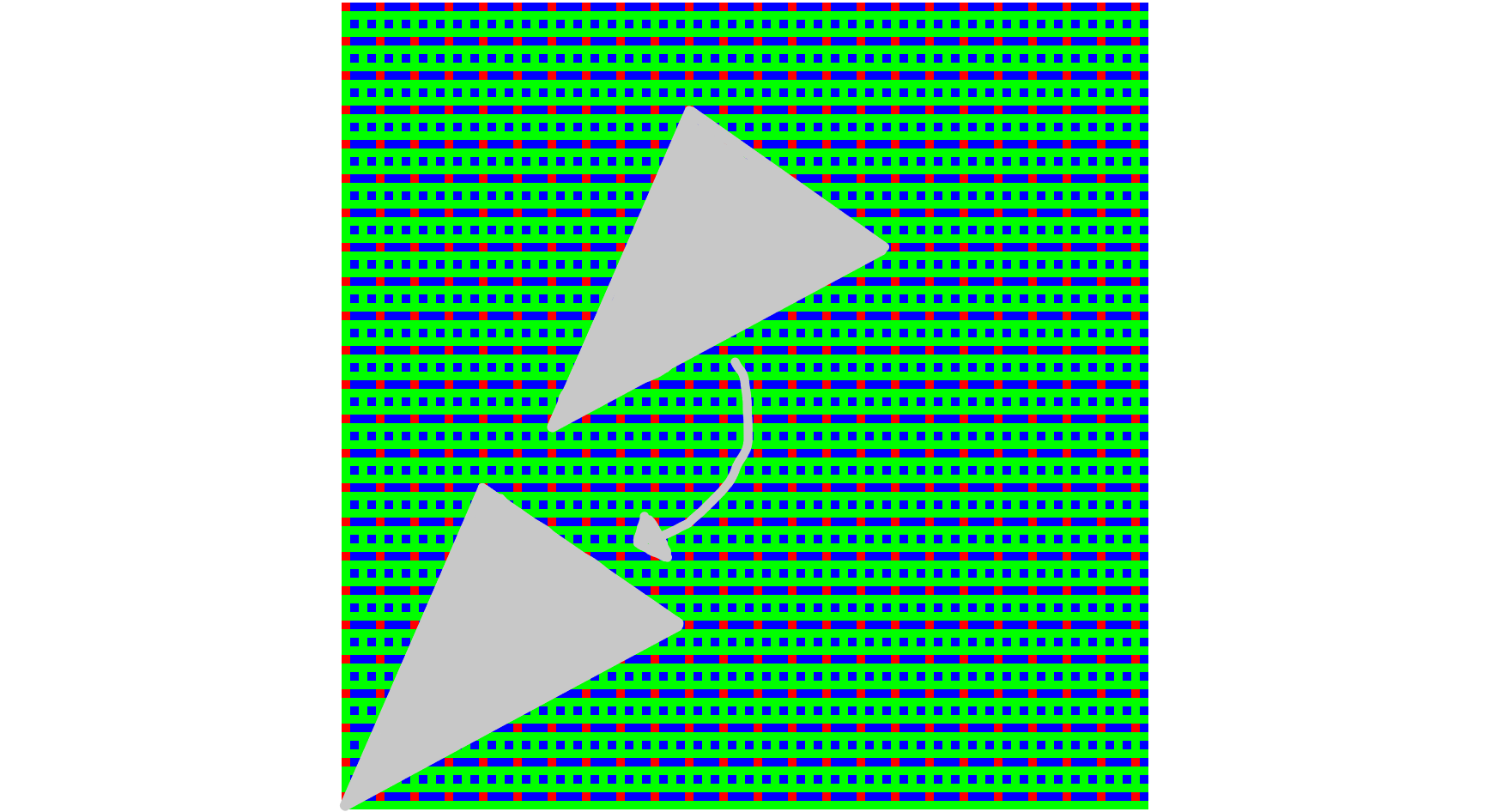
A graph is just a collection of nodes and edges that connect those nodes - each edge is between exactly \(2\) nodes. Graphs are essentially like a mathematical representation of a network. They look something like this:
A simple graph
The degree of each node (sometimes called \(\text{deg}(n)\)) is equal to the number of edges that come out of it. So, for example, node \(1\) has degree \(4\), while node \(2\) has degree \(1\).
Despite their simplicity, graphs have a surprising amount of depth to them - the entire field of graph theory is dedicated to studying these objects. One of the simplest theorems in graph theory is the handshake lemma, which states that the sum of the degrees of every node in a graph is equal to twice the number of edges in the graph.
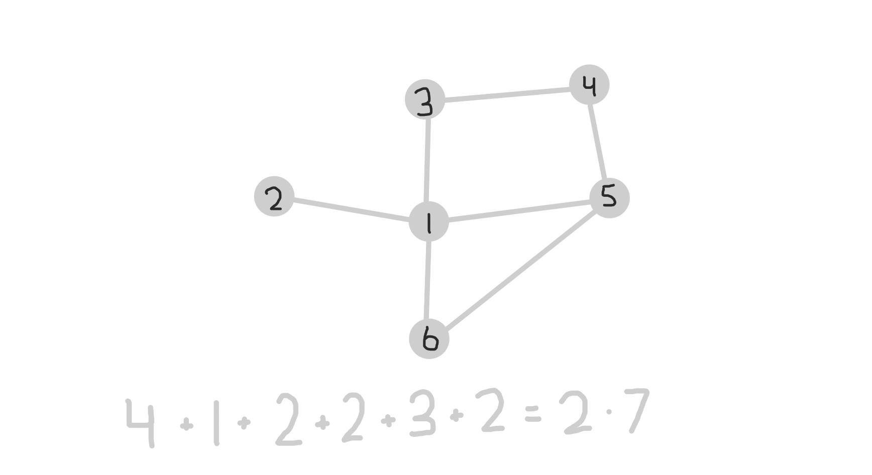
An example of the handshake lemma.
The proof is actually surprisingly simple - all we have to do is count the number of connections between nodes and edges from two different perspectives. Counting from the perspective of the nodes, each node contributes \(\text{deg}(n)\) connections by definition. However, counting from the perspective of the edges, each edge contributes exactly \(2\) connections. Since we’re counting the same quantity, we get our equality, as desired.
One of the most active subfields of graph theory is the study of colorings. It studies what we can learn from a graph if we give every node (or sometimes, every edge) a certain color.
Sound familiar? Well, it should! By coloring the entire real plane with \(3\) colors, we’ve essentially induced a coloring onto our triangulation, which means that we can study it using the tools of graph theory.
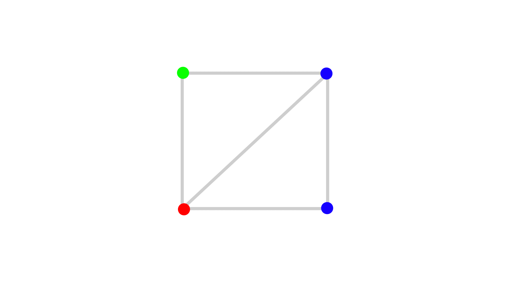
An example of a colored triangulation.
Now, it might not look like it right now, but we’re actually at a crossroads. There are two different ways to describe the triangulation with a graph. The first - which is more sensible at a first glance - is to have the nodes be the vertices of the triangles, and the edges be the edges of the triangles.
However, the alternative is to actually have the triangles themselves be the nodes. In this interpretation, two triangles would be connected to each other if they share an edge.
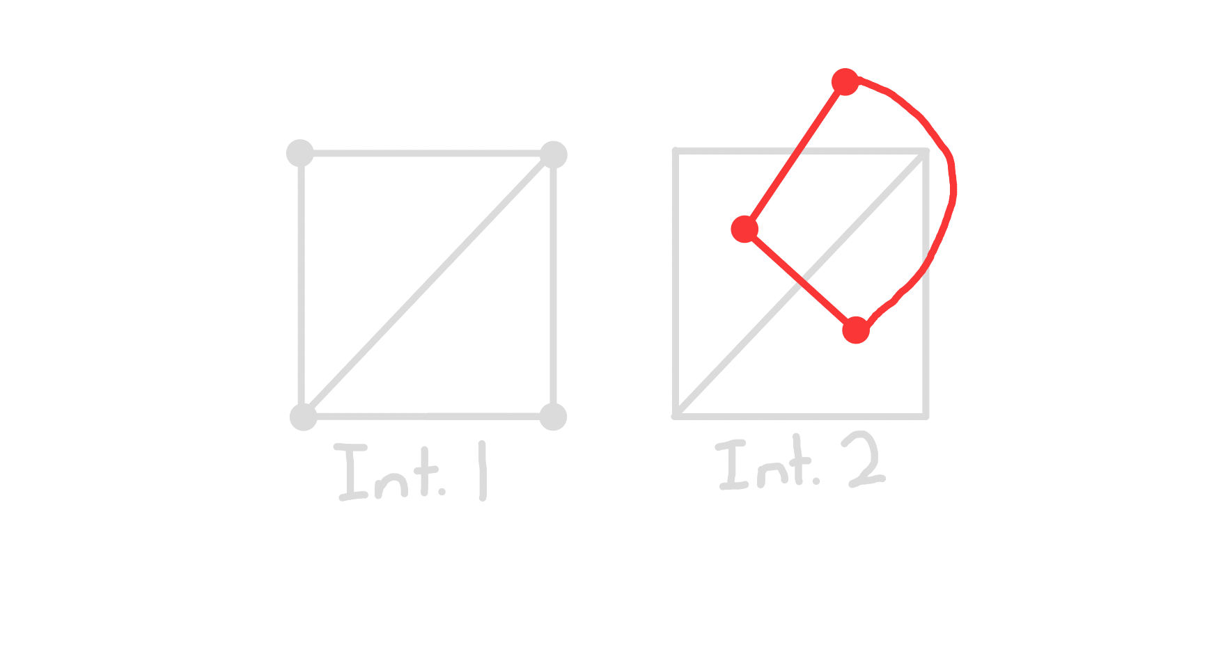
Two possible interpretations.
And yes, the outside of the square does count as a vertex. This graph is actually known as the “dual graph” of the first interpretation.
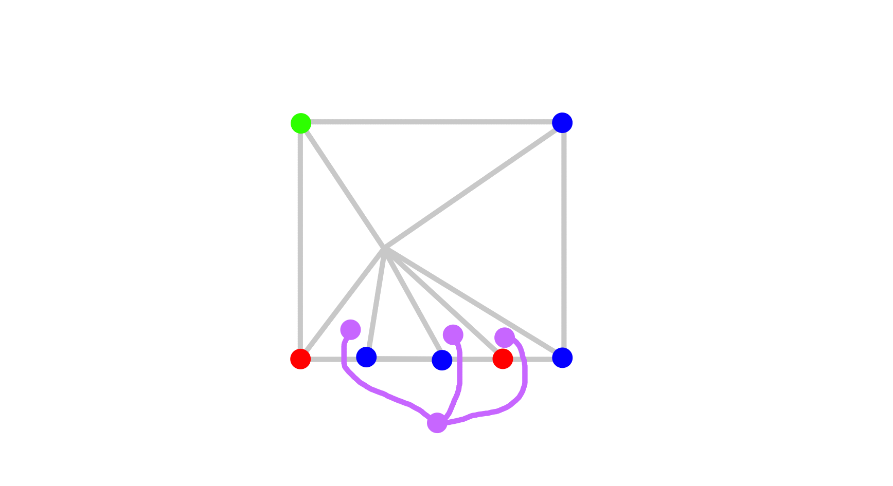
Now, the second method does have the drawback of not incorporating the colors of the vertices in any way. However, this can be fixed by coloring the connections of the graph depending on the colors of the vertices of the edges that connect two triangles (try saying that \(3\) times fast!). An example with only the blue-red edges connected is shown below.
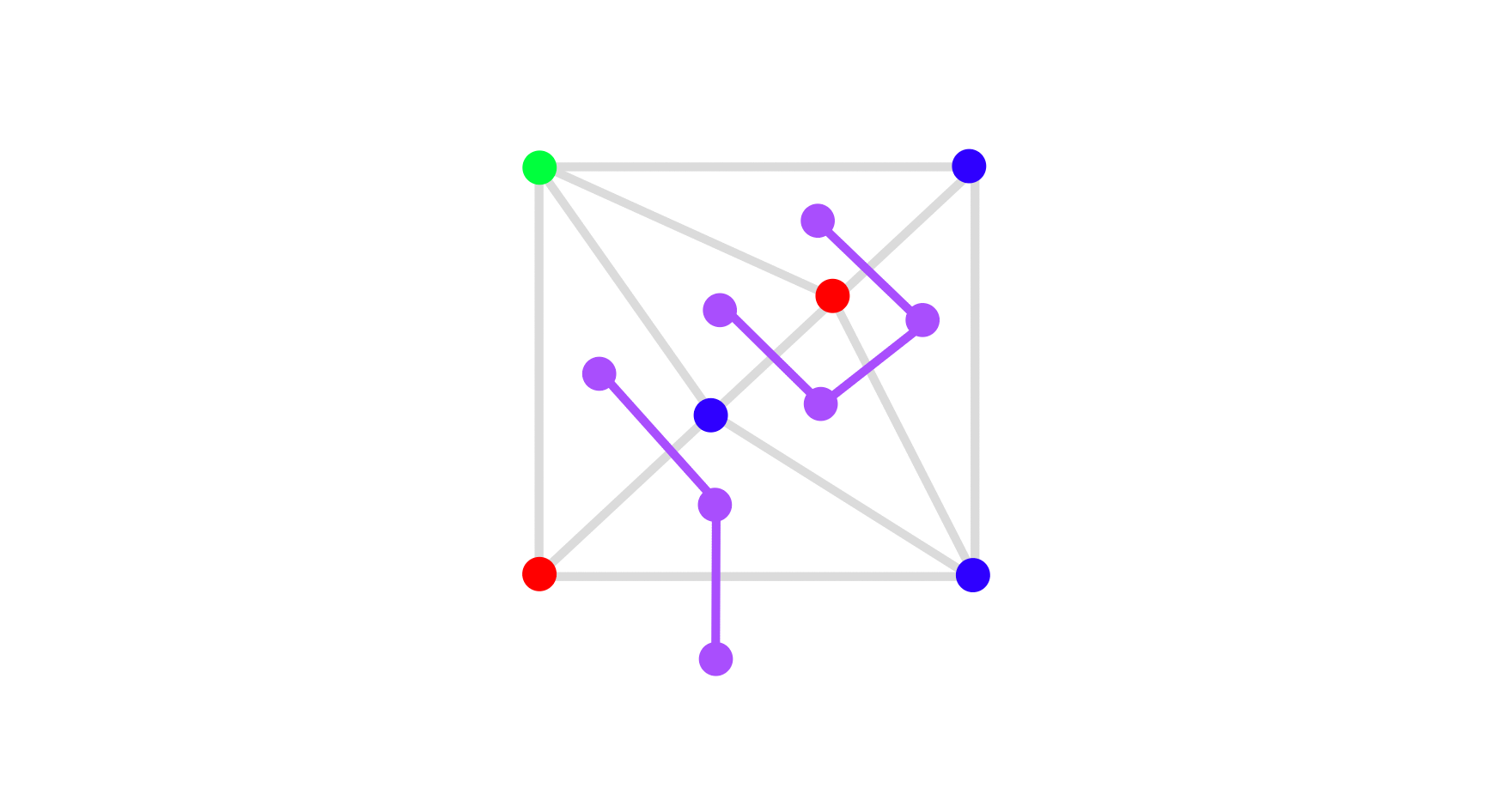
The dual graph with only red-blue edges counted.
As wrong as it feels, we’re going to be sticking to the second interpretation here. The basic reasoning is that our main objects of interest here are the triangles, not their constituent parts - as such, it would make more sense for the triangles to be the vertices, since it makes it easier for us to prove things about them.
So, how do we make progress from here? Well, one thing that we can notice pretty quickly is that there’s a pretty strict limit on what degrees the triangles can have - in fact, every triangle either has degree \(0, 1,\) or \(2\).
We can actually classify which triangles have which degrees! A triangle that has degree \(0\) cannot have any red-blue edges, and so must only be colored with \(2\) colors. A triangle that has degree \(2\) has \(2\) blue-red edges, and so must be colored only blue and red. A triangle that has degree \(1\), though, must have exactly one blue-red edge - and this means that the other vertex must be green. So, out of seemingly nowhere, we’ve found a description for our tricolor triangles!
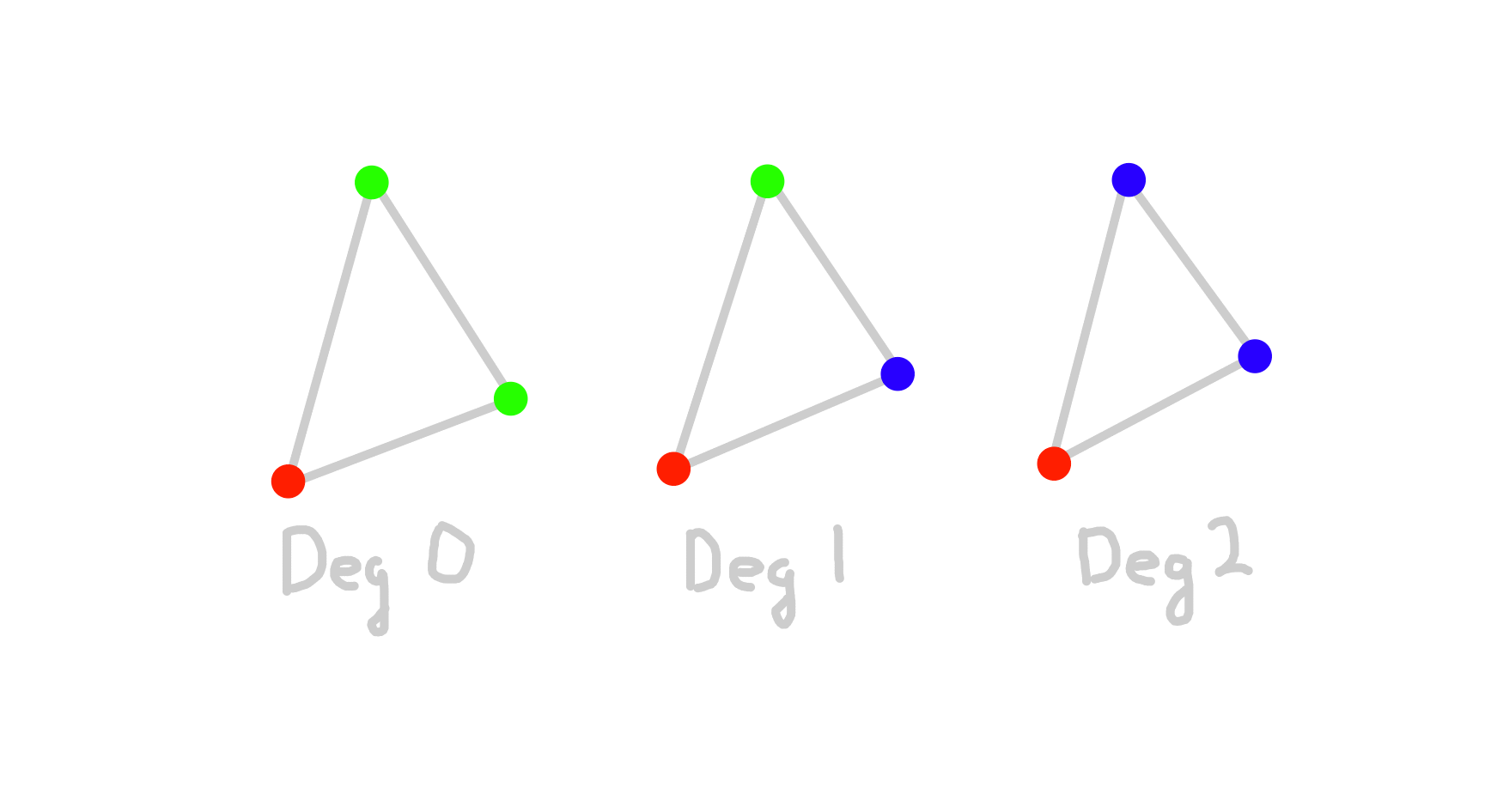
The 3 types of triangles.
What facts do we know about degrees? Well, one that comes to mind off the bat is the handshake lemma, which we proved earlier. The sum of the degrees of the triangles must be equal to twice the number of edges - more specifically, it must be even. Note that if the degree is \(0\) or \(2\), it doesn’t change the parity of the sum - that means that there has to be an even number of vertices with odd degree.
That means that if we can find at least \(1\) vertex with an odd degree, then we are done. This is actually where our “outside of the square” vertex comes in handy! We claim that this vertex has an odd degree. Note that the only connection the outside vertex can have with the inside of the square is through the bottom of the square.
Additionally, note that any point on the bottom of the square must be either blue or red - it can’t be green, because \(\|b\|_2 < 1\)! This implies that there must be an odd number of blue-red edges on the bottom line of the square - try splitting it up into different sequences of colors and seeing if you can figure out why.
The usefulness of the outside vertex.
So, that means that we have at least one vertex with odd degree, which implies that we must have at least one more. Since that vertex must be a triangle with degree \(1\), we have at least one tricolor triangle, as desired.
The astute among you might have noticed that nowhere here did we actually use the specific properties of the \(2\)-adic coloring! In fact, this property (known as Sperner’s lemma) holds for all colorings of the plane, as long as the shape we want to triangulate has exactly an odd number of blue-red borders.
So, we’ve now proven that every triangulation has at least one tricolor triangle. This triangle can be shifted to the origin without changing the colors of the vertices, which means that the other two vertices are blue and green. Then, computing the area of the triangle and using \(2\)-adic valuation, we see that the \(2\)-adic norm of the area must be greater than or equal to \(1\) - since \(\|\frac{2}{n}\|_2 = \frac{1}{2}\) for all odd \(n\), we have finally proved Monsky’s theorem.
5. Conclusion
So, there you have it! We’ve traveled from a simple geometry problem, to the land of \(p\)-adic analysis, all the way over to graph theory, and now we’ve finally proved the theorem.
Where do we go from here? Well, squares aren’t the only things that we can dissect into triangles. In fact, the initial discovery of Monsky’s theorem back in the late 1960s spawned an entire group of similar problems focused on equidissecting other polygons. Most of these problems use very similar tactics to the problem we looked at today - \(p\)-adic colorings of the real numbers and Sperner’s lemma (or extended versions of it) are the two primary tools.
For now, though, I think I’ll just invite another person to my birthday party.