1. Introduction
A couple years ago - back when I still coded things - I stumbled across a seemingly-innocent problem in computer science about permuting matrices of numbers. Initially, I thought the problem just needed a little algorithmic speedup in order to work; however, the deeper I dived, the more I realized how mathematical the structure behind this problem was.
In the end, my solution was actually primarily mathematical, drawing from group-theoretic ideas to optimize the algorithm. This problem means quite a lot to me, because it was one of the first times I actually applied higher mathematics to a non-mathematical problem, and I think it’s one of the reasons why I love math as much as I do today.
The problem is as follows: Let \(M\) be the set of all \(w \times h\) matrices whose elements are drawn from the set \(\{1, \dots, n\}\), and let \(S\) be a subset of \(M\) such that no element of \(S\) can be rearranged into another one by permuting its rows and columns. Given \(w, h,\) and \(n\), compute the largest possible size of \(S\).
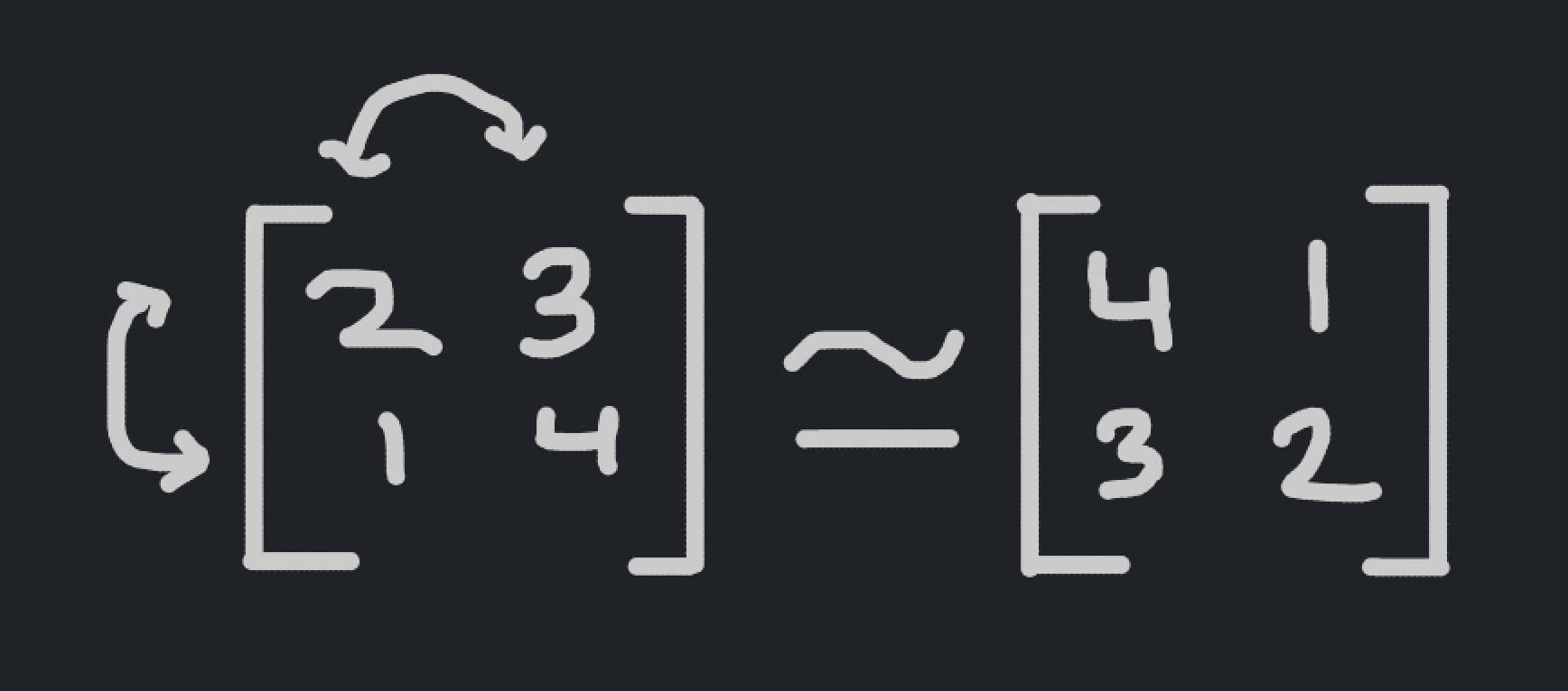
An example of two matrices that can be permuted to equal each other.
Through the rest of this blogpost, I’ll walk you through my solution to the problem. Along the way, we’ll make some clever connections to Burnside’s Lemma and group theory, and we’ll end up with an efficient algorithm that is magnitudes faster than the naive approach.
Let’s get started.
2. A Naive Attempt
As with any computer science problem, the naive approach here is to simply brute-force all possible matrices in \(M\), greedily adding them to our set \(S\) until we can’t add a matrix anymore. This wil give us the optimal size of \(S\) - while that’s a little hard to prove at this point, you’ll later see that this is because we’re simply selecting an element of each “orbit” of the matrices under permutation; I’ll explain what that means in a future section.
The problem with this approach, though, is that it takes a long time. For the computer scientists in the audience, it should be pretty easy to see that this algorithm has runtime \(O(n^{wh})\); and for those of you that don’t know what that means, it’s essentially any developer’s nightmare. This kind of exponential runtime means that even with relatively small values of \(w, h,\) and \(n\), the algorithm will take enormous amounts of time to run. For the constraints provided in the original problem: \(w, h \leq 12\), and \(n \leq 20\), the algorithm could take up to \(20^{135}\) seconds to run, assuming that checking whether two matrices are equivalent under permutation takes just one nanosecond. This is longer than the age of the universe squared: not the most efficient algorithm, if you can’t tell.
The universe has been around for a pretty long time.
There are some basic speedups that you can make to optimize this naive algorithm; for example, if two matrices differ in their elements, then they obviously cannot be permuted to form one another. However, even with these speedups, you have an insane amount of matrices to check, and the runtime doesn’t get much better.
The main problem with this approach is that it’s not taking advantage of the “structure” present in the problem. If we had some way to mathematically encode what it means to “permute” the columns and rows of a matrix, then we might be able to take advantage of this structure in order to speed up our algorithm.
That’s where group theory comes in.
3. Groups
Group theory is a mathematical way of encoding structure in an object called a group, which is an abstract mathematical object with specific properties. The beauty of groups is how they capture the basic structure behind many other mathematical objects; this means that an observation about groups is applicable across all kinds of mathematics.
Formally, a group is a set \(G\) of objects and an operation \(\cdot\) that is binary (that is, it takes two elements \(a, b\) in \(G\) and maps it to an element \(a \cdot b\) also in \(G\)) such that the following three group axioms are satisfied:
- The group operation is associative; that is, if \(a, b, c \in G\), then \(a \cdot (b \cdot c) = (a \cdot b) \cdot c\).
- There exists an identity element in \(G\); that is, there exists an element \(e \in G\) such that if \(a \in G\), then \(a \cdot e = a\).
- Every element of the group has an inverse; that is, for any \(a \in G\), there exists a corresponding element \(a^{-1} \in G\) such that \(a^{-1} \cdot a = a \cdot a^{-1} = e\).
These axioms aren’t very restrictive, and the majority of mathematical objects that mathematicians find interesting to study have some sort of group structure underlying them. As a basic example, the sets of real numbers, rational numbers, and integers are all groups with the group operation of addition. If you would like, you can check each of the group axioms for each of these groups, and you should be able to confirm that each of these sets are indeed groups.
Oftentimes, the element \(a \cdot b\) will simply be written as \(ab\); in later sections, \(\cdot\) will be used to denote a different operation.
The integers are a group under addition.
That being said, the set of natural numbers is not a group with the group operation of addition. Can you see why not?
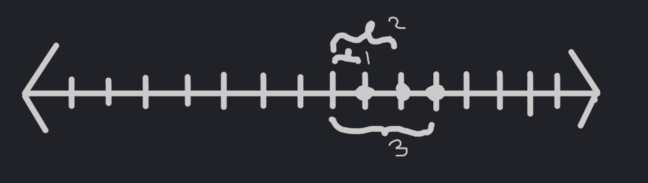
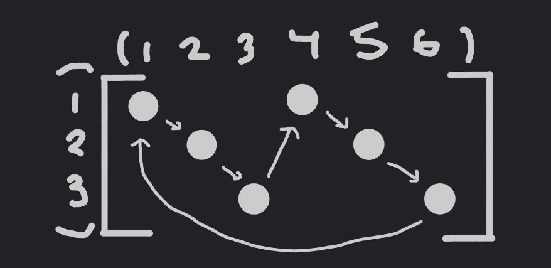
One type of group that will be very useful to us later on is the permutation group \(S_n\), which consists of the set of permutations of the sequence \(\{1, \dots, n\}\). Alternatively, it can also be described as the set of bijective functions from the set \(\{1, \dots, n\}\) to itself. The group operation of this group is conjugation: so you apply one permutation to the sequence, and then the next.
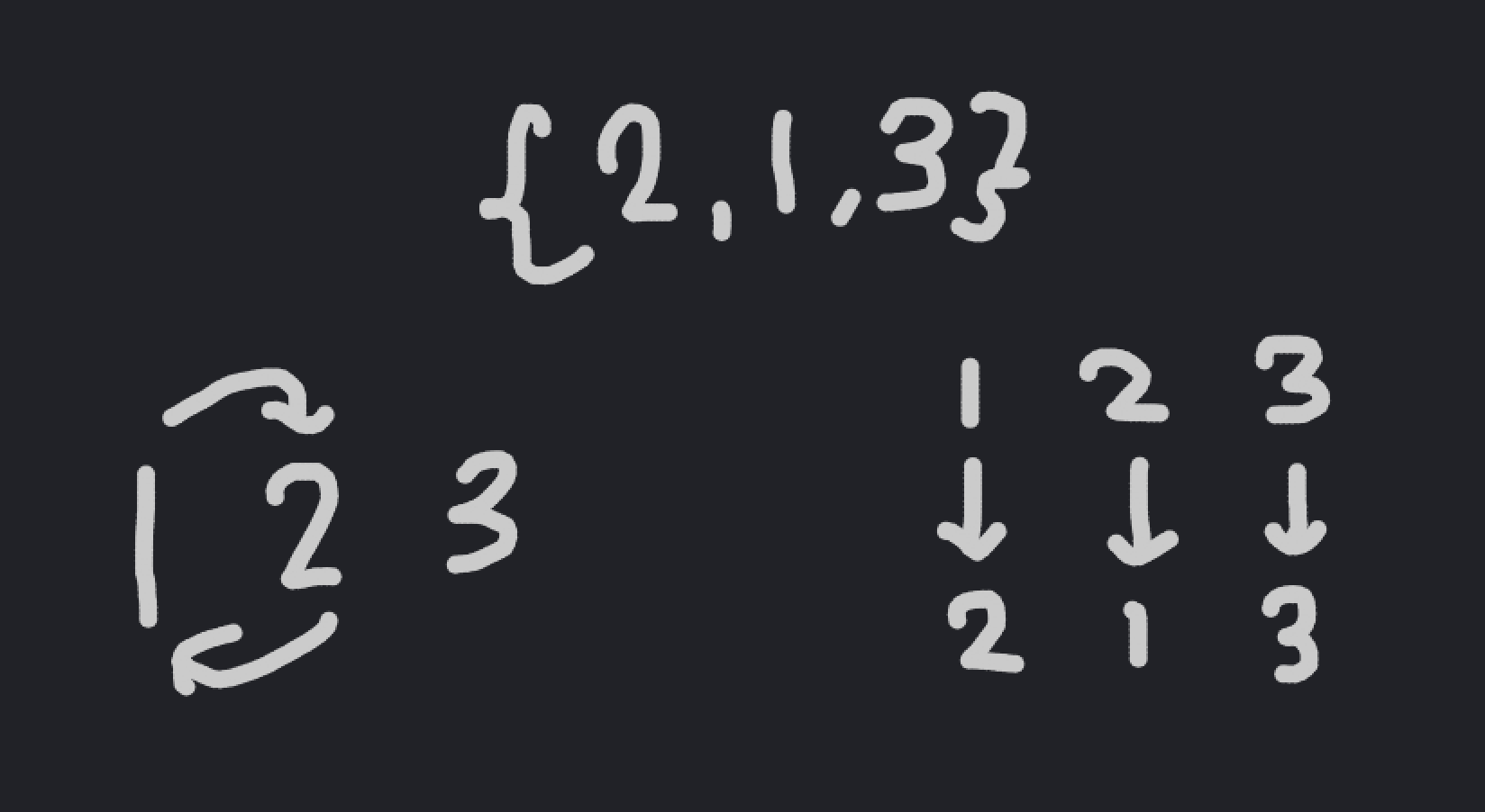
The two interpretations of a permutation.
We often note a permutation as a result of applying it to the base sequence \(\{1, \dots, n\}\); for example, the permutation \(\{2, 1, 3\}\) just swaps the first two elements of the sequence. Arbitrary permutations are often denoted by \(\sigma \in S_n\).
We can manually check that this is indeed a group, since it satisfies the three group axioms:
- The group operation is associative, since in both \(\sigma_1 \circ (\sigma_2 \circ \sigma_3)\) and \((\sigma_1 \circ \sigma_2) \circ \sigma_3\), you’re applying all three permutations in the same order.
- The identity is just the permutation that takes \(\{1, \dots, n\}\) to \(\{1, \dots, n\}\).
- The inverse of a permutation just takes the elements back to where the started. So, if \(\sigma \in S_n\) takes \(\{1, \dots, n\}\) to \(\{\sigma(1), \dots, \sigma(n)\}\), then the inverse permutation \(\sigma^{-1}\) takes \(\{\sigma(1), \dots, \sigma(n)\}\) to \(\{1, \dots, n\}\).
There are a lot of interesting facets to the permutation group \(S_n\) that make it a nice object to study, in terms of structure. Some of these facets will be discussed later in the post.
The astute among you, though, might have noticed that our set \(M\) from the problem isn’t actually a group. In fact, it’s completely unclear how we would even turn it into a group; there’s just no obvious way of defining a group operation over the matrices.
How would you form a group over these matrices?
So, is group theory a dead end? The answer is no. In fact, we can see that the permutations of rows and columns discussed in the problem look very similar to the permutation groups we just talked about above.
If we could find a way to apply these permutation groups to a set of objects, then we would finally have our desired mathematical description of the problem. That’s where group actions come into play.
4. Group Actions
A group action is a way of studying how a set behaves when the group “acts” on it.
Formally, given a group \(G\) and a set of objects \(X\), a group action of \(G\) on \(X\) is a new binary operation \(\cdot\), where the left input comes from \(G\) and the right input comes from \(X\), which satisfies the following properties:
- If \(e\) is the identity element of \(G\), then \(e \cdot x = x\) for any \(x \in X\).
- If \(g, h \in G\) are elements of the group, then \((gh) \cdot x = g \cdot (h \cdot x)\).
An example would likely make this more clear, since it’s a little confusing on it’s own. Let \(X\) be the set of sequences of length \(6\), where each element is chosen from the set \(\{1, \dots, 6\}\) - this corresponds to our problem in the case \(w = 1, h = 6, n = 6\). Then, let \(G\) be the permutation group \(S_6\); there is a natural group action of \(G\) on \(X\) that simply permutes the elements of the sequence in \(X\).
An example of a group action.
Besides the definition of a group action, there are some other definitions that we need to know before we can move onto the meat of the problem. Firstly, we need to define the fixed points of a group action. For an element \(g \in G\), an element \(x \in X\) is said to be a fixed point of \(g\) if \(g \times x = x\). We often denote the set of all fixed points of \(g\) in \(X\) as \(X^g\).
Returning to our previous example, we can consider the element of the group \(\sigma = \{1, 2, 3, 4, 6, 5\}\). What are the fixed points of this element in \(X\)?
If \(x = \{x_1, \dots, x_6\}\) in \(X\), then \(\sigma \cdot x = \{x_1, x_2, x_3, x_4, x_6, x_5\}\). For us to have \(g \cdot x = x\), then we need to have \(x_5 = x_6\), and that is the only requirement. For example, \(\{1, 2, 3, 4, 5, 5\}\) is a fixed point of \(\sigma\).
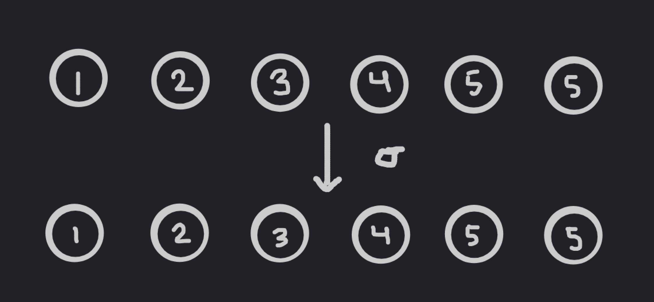
An example of a fixed point.
A related idea is orbits. The orbit of an element \(x \in X\) is the set formed by \(g \cdot x\) for any \(g \in X\).
For example, let’s try to find the orbit of the element \(x = \{1, 1, 1, 1, 1, 2\}\). Any permutation \(g \cdot x\) of \(x\) can swap the two with any of the ones, and that’s actually all it can do, since it can’t affect the actual elements of \(x\) in any way. This tells us that the orbit of \(x\) is just the set of all sequences with one \(2\) and five \(1\)s.
It can be seen relatively easily that orbits are disjoint from each other; that is, if an element \(a\) is in the orbit of \(x\), and \(a'\) is not in the orbit of \(x\), then \(a'\) cannot be in the orbit of \(a\). In other words, the orbits of a group action divide the set into a group of equivalency classes. The number of orbits of a group action is often denoted as \(\| X / G\|\).
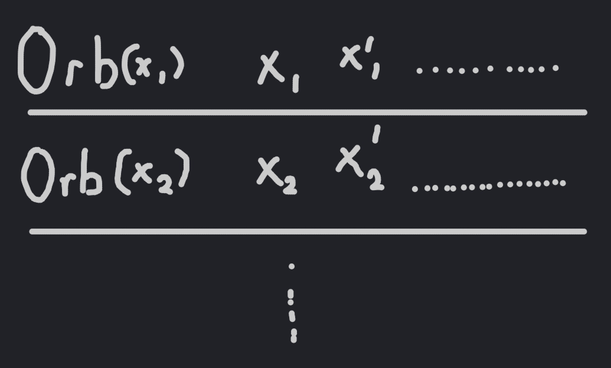
Orbits form equivalence classes over a set.
At this point, it might start becoming clear how we would apply the concept of group actions to our problem. The permutations of the columns of our matrix can be represented as \(S_w\), since there are \(w\) columns. Similarly, the permutations of the rows of our matrix can be represented as \(S_h\). The actual details aren’t super important, but the combination of the two can be represented by the product group \(S_w \times S_h\); this is just the group formed by the elements \((\sigma, \tau)\), where \(\sigma \in S_w\) and \(\tau \in S_h\), where the group operation is defined by \((\sigma_1, \tau_1)(\sigma_2, \tau_2) = (\sigma_1 \sigma_2, \tau_1 \tau_2)\).
Then, we would have to consider the group action of \(S_w \times S_h\) on our set of matrices \(M\). The group operation is defined naturally: the element \((\sigma, \tau) \in S_w \times S_h\) first applies the permutation \(\sigma\) to the columns of the matrix, and then applies \(\tau\) to the rows. Note that it doesn’t actually matter what order we apply the two permutations in; if you don’t believe me, you can try to prove it by yourself. It’s relatively simple.
How do our concepts of orbits and fixed points relate to this problem? Well, note that if two elements of \(M\) are in the same orbit, then they cannot both be in the set \(S\) defined in the problem. That’s because if they’re in the same orbit, then there must exist a permutation in \(S_w \times S_h\) that takes the first element to the second one, which goes against the constraints of the problem.
Similarly, if two elements aren’t in the same orbit, then they can always both fit in our subset \(S\), since by definition, there’s no permutation of rows and columns that takes the first element to the second one.
To get the largest possible subset, select an element from each orbit.
To get the largest possible subset \(S\), then, we simply have to select one element of each orbit of the group action. In other words, to compute the size of \(S\), we need to compute the number of orbits \(\| M / (S_w \times S_h)\|\).
Luckily for us, group theory gives us a tool to do just that.
5. Burnside’s Lemma
Burnside’s Lemma gives us a way to compute the number of orbits using the number of fixed points of every element in the group action. More specifically, the lemma states that:
$$\| X / G\| = \frac{1}{\| G\|} \sum_{g \in G} \| X^g\|$$
In English, that means that the number of orbits of the group is equal to the average number of fixed points of elements in the group.
The proof of Burnside’s Lemma is quite interesting, and relies on something known as the Orbit-Stabilizer Theorem. If you’re familiar with group theory, but not with group actions, I recommend checking the proof out; it is neat.
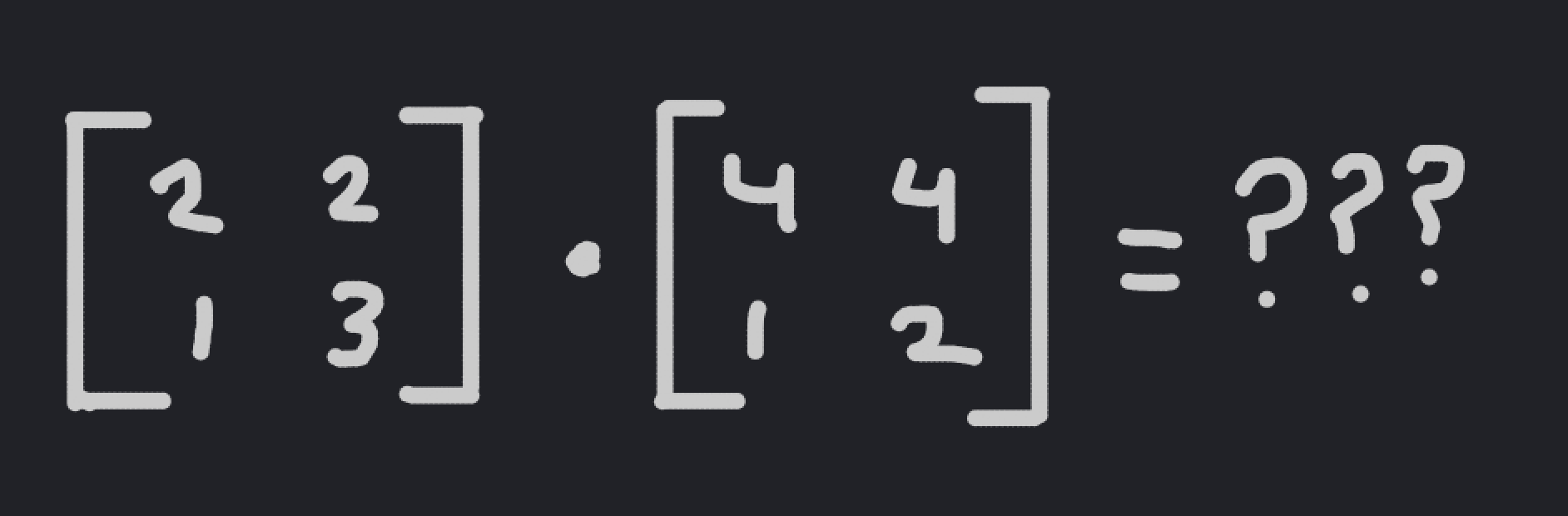
Before we apply Burnside’s Lemma to our problem, let’s do a simple example with it to demonstrate its power. Say that we have six indistinguishable balls, and we want to place them into three indistinguishable boxes. How many unique ways are there to do this?

An example configuration of balls placed in bins.
While this problem is relatively easy to attack using basic casework, we can also apply Burnside’s Lemma to it. Consider the number of arrangements of six indisinguishable balls into three distinguishable boxes, and let this be a set \(X\). Then, we can consider the set \(S_3\) acting on the three boxes; we claim that our desired answer is the number of orbits \(\| X / S_3\|\). Indeed, note that if two arrangements are in the same orbit, then they correspond to the same configuration, since if the boxes were indistinguishable, we could simply move them around as we wished.
To do this, we can apply Burnside’s Lemma, which states that
$$\| X / S_3\| = \frac{1}{6} \sum_{\sigma \in G} \| X^\sigma\|$$
We can compute the number of fixed points of each permutation by hand. I won’t do all of the work here, since it’s long and quite tedious; if you’d like, you can check out the example at [this]{https://brilliant.org/wiki/burnsides-lemma/} link. In summary, though, you end up getting
$$\| X / S_3\| = \frac{1}{6} (28 + 4 + 4 + 4 + 1 + 1) = 7$$
which matches what you get when you write out each permutation by hand.
In this case, the computation of the fixed points is a little difficult, so Burnside’s Lemma isn’t the most efficient way to solve the problem. Still, though, it’s a nice demonstration of the duality between fixed points and orbits that Burnside’s Lemma attempts to capture.
Now, let’s return to the problem at hand. Using Burnside’s Lemma, we get the equality
$$\| M / (S_w \times S_h)\| = \frac{1}{\| S_w \times S_h\|} \sum_{(\sigma, \tau) \in S_w \times S_h} \| M^{(\sigma, \tau)}\|$$
Now, what’s left is to count the fixed points of a given permutation.
6. Finding Fixed Points
Our general approach to finding the fixed points of a permutation will be as follows: we’ll “relabel” the permutation in a way that maintains the fixed points, which will allow us to reduce everything to a simple case that we can analyze directly. Before we can figure out how to relabel our points, though, we need to learn about some additional properties of the permutation group \(S_n\).
There is another way to write a permutation in \(S_n\) known as cycle notation. Cycle notation, as you might be able to imagine, writes a permutation in terms of its cycles, instead of just examining how it affects the sequence \(\{1, \dots, n\}\).
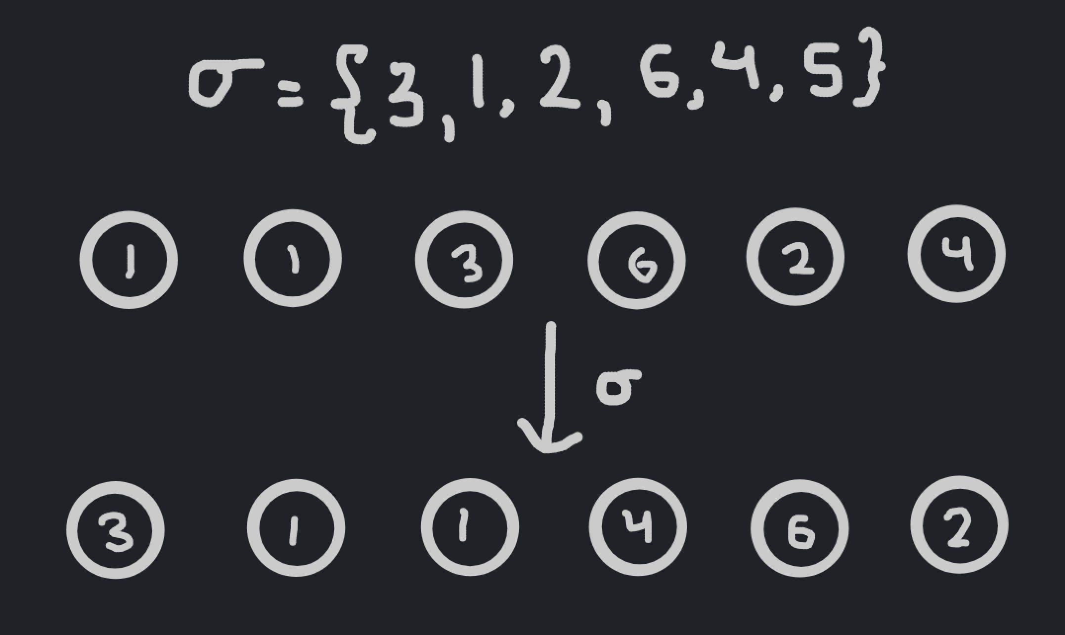
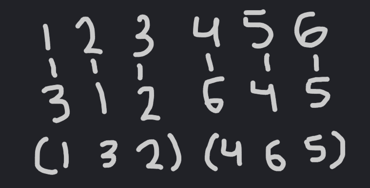
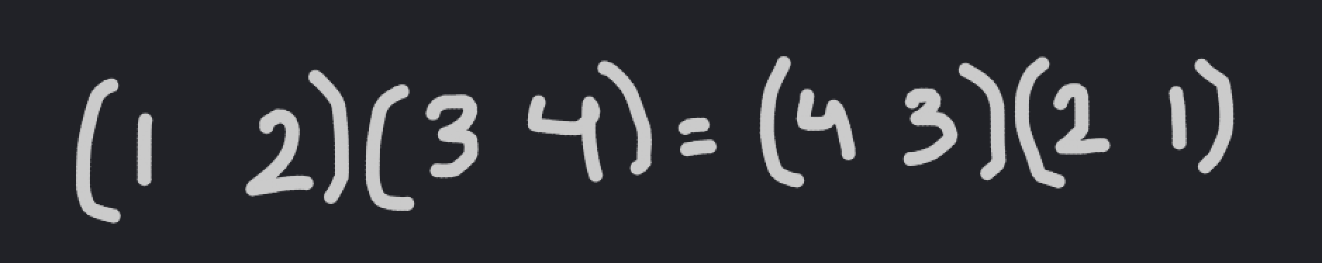
For example, consider the permutation \(\sigma = \{3, 1, 2, 6, 4, 5\}\) in \(S_6\). To write it in cycle notation, we can just follow where each element goes when the permutation is applied. For example, the first number in the permutation is \(3\), so the permutation maps \(1\) to \(3\). Then, the third element is \(2\), so the permutation maps \(3\) to \(2\). Finally, the second element is \(1\), so the permutation maps \(2\) to \(1\).
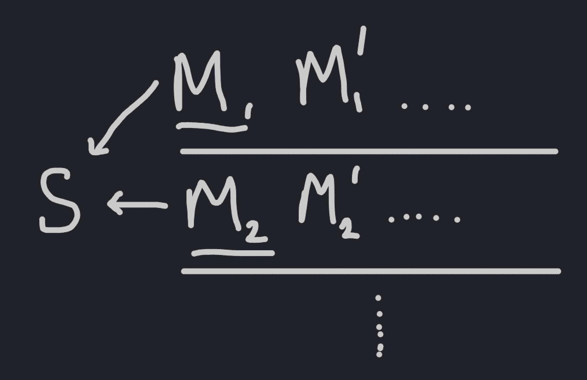
In other words, there exists a cycle \((1, 3, 2)\) in the permutation. There is also another cycle that you could find; it is \((4, 6, 5)\). Therefore, in cycle notation, we have \(\sigma = (1, 3, 2)(4, 6, 5)\).
On the top is the regular interpretation of a permutation; on the bottom, it's in cycle notation.
To go back from cycle notation to the regular notation, we just have to “follow” each cycle to reconstruct our original permutation. Note that it doesn’t matter what order in which you write your cycles; since all cycles are distinct, and all will end up being applied to your permutation.
The cycle notation of a permutation gives a natural “cycle structure” to the permutation, based on the size of each cycle. For example, we could say that the \(\sigma\) above has cycle structure \((3, 3)\), since those are the sizes of the two cycles in the permutation.
It’s relatively easy to see that the cycle structures in \(S_n\) correspond to the partitions of \(n\), by just making a cycle of length \(k\) for every integer \(k\) in the partition. For example, the partition \(6 = 3 + 3\) corresponds to the cycle structure \((3, 3)\).
So, why bring up cycle notation? Well, as it turns out, any two permutations that have the same cycle structure will have the same number of fixed points!
This is because if two permutations in \(S_w\) have the same cycle structure, then we can relabel the columns of the matrix \(M\) to get from one permutation to the other.
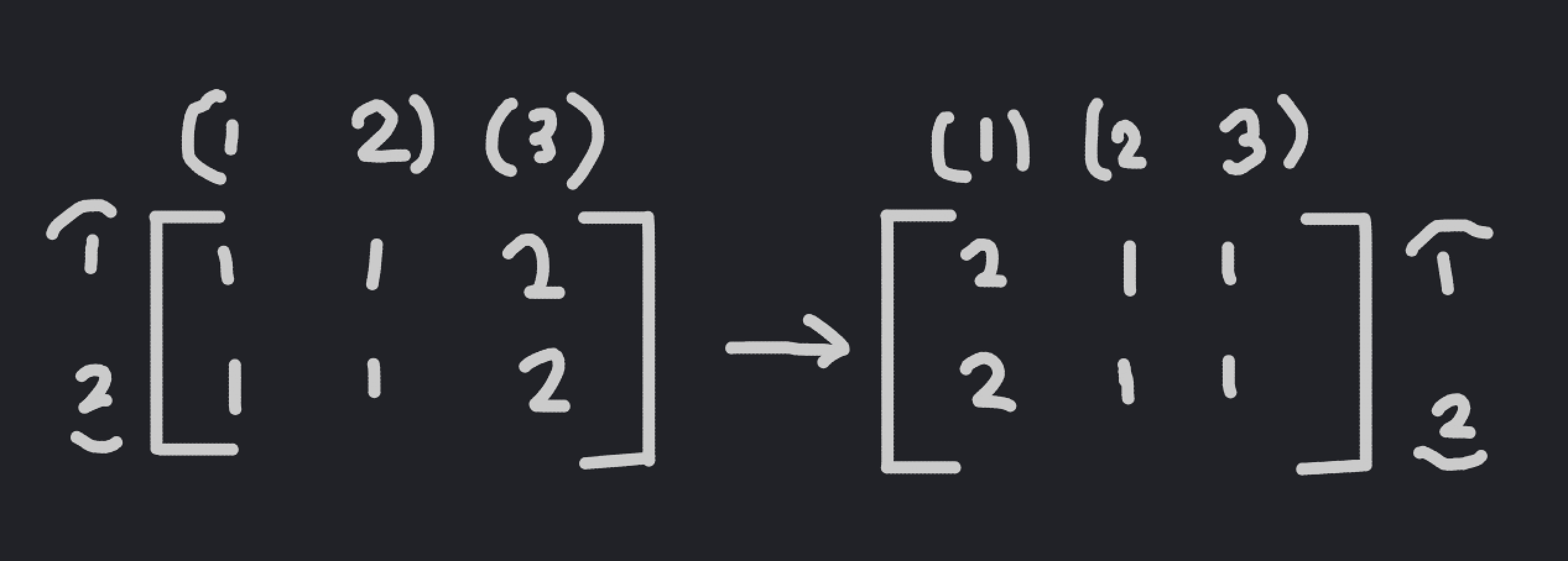
An example relabeling. Note that this is a fixed point of the new permutation.
Note that this relabeling uniquely maps one fixed point of the first permutation to a fixed point of the second permutation; if a matrix \(M_1\) is a fixed point of the first permutation, then the relabeled matrix \(M_2\) is a fixed point of the second permutation. Since it is a bijective map, both permutations have the same number of fixed points.
When considering both dimensions instead of just one, it’s not much more complicated. If the cycle structures of both parts of an element \((\sigma, \tau) \in S_w \times S_h\) are the same, then the two elements have the same number of fixed points in \(M\).
Later on, we’ll have to use the number of permutations that correspond to each cycle structure, so we compute that quantity now. Say that we wanted to compute the number of permutations in \(S_w\) that have cycle structure \((a_1, \dots, a_k)\) where \(a_1 + \dots + a_k = w\). First, note that we can place the elements of the sequence \(\{1, \dots, w\}\) into the cycle structure in any order to get a permutation; we simply have to account for the fact that this overcounts some of the permutations.
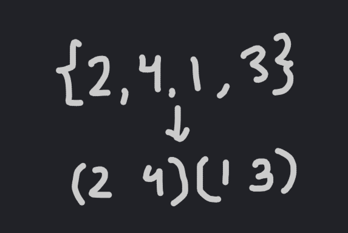
An example of placing numbers into a cycle structure to get a permutation.
For the first cycle of length \(a_1\), there are \(a_1\) ways to represent the cycle; this is because pushing forward each element of the cycle by one keeps the cycle the same. Additionally, if two of the cycles have the same size, then we have to account for permuting the two cycles with one another, and we’d have to do similar things with any number of cycles of the same size.
Two ways of writing the same permutation in cycle notation.
That was a little complicated, so let’s do an example. Say we wanted to find the total number of permutations with cycle structure \((3, 2, 2, 1)\). Then, we divide \(8!\) by \(3 \cdot 2 \cdot 2 \cdot 1 \cdot 2! = 24\); \(3, 2, 2, 1\) correspond to the overcounting in the individual cycles, and \(2!\) accounts for the overcounting since there are two cycles of the same size.
Now, we can compute the fixed points of every cycle structure. Since we have the choice of which permutation to select for each cycle structure, we can simply select the most basic one; for example, for the cycle structure \((3, 2, 1)\), we can select the permutation \((1, 2, 3)(4, 5)(6)\) in \(S_6\). Then, the movement of a matrix under our permutation actually becomes really easy to analyze; it simply shifts each row and column of the matrix in a cycle, as shown.
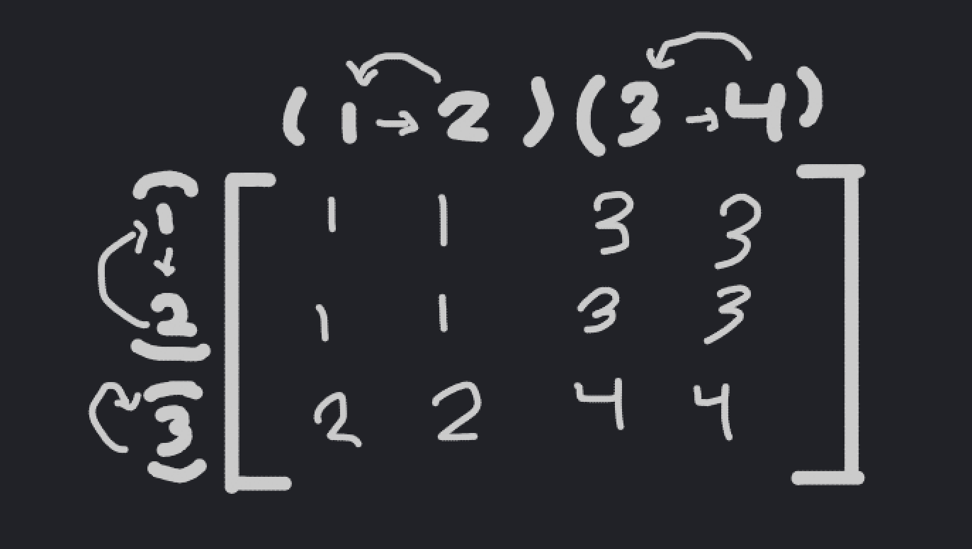
An example permutation of the matrix.
Note that the permutations seperate the matrix into smaller “rectangles”, which don’t affect one another. Therefore, a fixed point of the full matrix must be a fixed point of the individual rectangles.
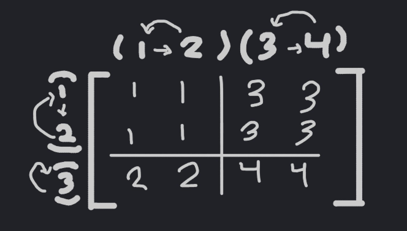
An example permutation of the matrix, split into rectangles.
Therefore, it simply remains to compute the fixed point of a rectangle. Say that we’re looking at a rectangle with width \(a\) and height \(b\). To find a fixed point of the rectangle, we can examine how each element moves under the permutation. As it turns out, each application of the permutation will move an element of the matrix down one and to the right one, by definition. Once the elements reach the edge of the matrix, they simply cycle around to the top (or left) of the matrix, respectively.
Pick an element of a random fixed point of the permutation. Since it’s a fixed point, if we apply the permutation, we should get the same matrix back. Therefore, the point that the element maps to must be the same as the original element, if the matrix is a fixed point.
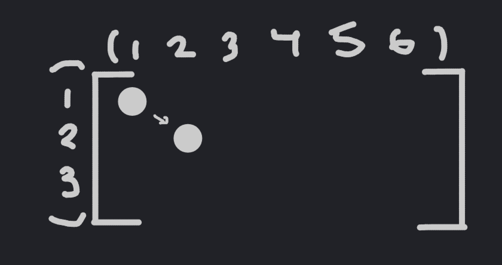
The movement of an element under a single permutation of the rectangle.
Then, we can just apply the permutation to the matrix multiple times. Each time, it must be the same as the original matrix, so we get a collection of elements that must be equal to our original element.
The movement of an element under multiple permutations of the rectangle.
Note that this seperates the matrix into multiple collections of elements of the matrix, all of which must be equal in order for the original matrix to be a fixed point. Then, we can simply select an member of \(\{1, \dots, n\}\) to assign to all of those elements, and there are \(n\) ways to do this. It is relatively simple to show that there are a total of \(\text{gcd}(a, b)\) collections of elements that must be equal; if you would like to prove it, try assigning coordinates to the elements of the matrix such that the sum of the coordinates stays the same under permutation.
7. Putting it All Together
Now, we have all the parts we need in order to compute the number of orbits of our original class. The process goes as follows:
- Compute the number of cycle structures in \(S_w\) and \(S_h\) by finding their partitions.
- For every set of cycle structures, compute the number of fixed points of their representative permutations.
- You can do the above by computing the number of fixed points of every constituent “rectangle” of the matrix, and multiplying the results in order to get your answer.
- Finally, multiply the number of permutations of each cycle structure, and sum across all cycle structures to finish.
$$\| M / (S_w \times S_h)\| = \frac{1}{w!h!} \sum_{(a_1, \dots, a_k) \in \mathcal{P}_w} \sum_{(b_1, \dots, b_\ell) \in \mathcal{P}_h} f(a_1, \dots, a_k)f(b_1, \dots, b_\ell) \prod_{i=1}^k \prod_{j=1}^\ell n^{\text{gcd}(a_i, b_j)}$$
where \(\mathcal{P}_w, \mathcal{P}_h\) are the sets of partitions of \(w\) and \(h\), respectively, and \(f(a_1, \dots, a_k)\) is the number of permutations in \(S_w\) with cycle structure \((a_1, \dots, a_k)\), which we described how to compute earlier. This is a really complicated formula, if you’re a human; however, for a computer, evaluating a formula like this is a piece of cake.
8. Conclusion
As promised, this algorithm is much faster than the original algorithm. The only real time-consuming step in this algorithm is computing the number of partitions of \(w\) and \(h\), which is an exponential evaluation at worst. This is much better than the \(O(n^{wh})\) algorithm that we started with. In fact, even with the maximal constraints, this algorithm ran in approximately \(0.35\) seconds on my local machine in Python 2.7, which is a much better time complexity than the age of the universe squared.
More important than the computational speedup, though, is how this solution was found. The way that Burnside’s Lemma, an idea from group theory, could be used to tackle this seemingly-unrelated computer science problem is something I found incredibly interesting.
I hope you enjoyed this problem as much as I did.